Getting started

This tutorial is based on the quickstart example in the celerite documentation, but it has been updated to work with celerite2.

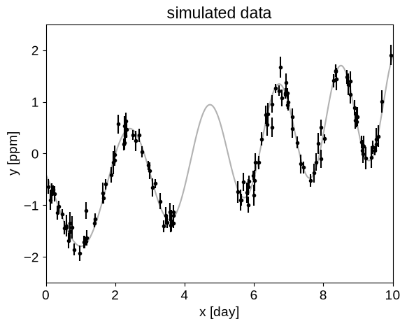
For this tutorial, we’re going to fit a Gaussian Process (GP) model to a simulated dataset with quasiperiodic oscillations. We’re also going to leave a gap in the simulated data and we’ll use the GP model to predict what we would have observed for those “missing” datapoints.

To start, here’s some code to simulate the dataset:

import numpy as np
import matplotlib.pyplot as plt

np.random.seed(42)

t = np.sort(
    np.append(
        np.random.uniform(0, 3.8, 57),
        np.random.uniform(5.5, 10, 68),
    )
)  # The input coordinates must be sorted
yerr = np.random.uniform(0.08, 0.22, len(t))
y = (
    0.2 * (t - 5)
    + np.sin(3 * t + 0.1 * (t - 5) ** 2)
    + yerr * np.random.randn(len(t))
)

true_t = np.linspace(0, 10, 500)
true_y = 0.2 * (true_t - 5) + np.sin(3 * true_t + 0.1 * (true_t - 5) ** 2)

plt.plot(true_t, true_y, "k", lw=1.5, alpha=0.3)
plt.errorbar(t, y, yerr=yerr, fmt=".k", capsize=0)
plt.xlabel("x [day]")
plt.ylabel("y [ppm]")
plt.xlim(0, 10)
plt.ylim(-2.5, 2.5)
_ = plt.title("simulated data")

Now, let’s fit this dataset using a mixture of SHOTerm terms: one quasi-periodic component and one non-periodic component. First let’s set up an initial model to see how it looks:

import celerite2
from celerite2 import terms

# Quasi-periodic term
term1 = terms.SHOTerm(sigma=1.0, rho=1.0, tau=10.0)

# Non-periodic component
term2 = terms.SHOTerm(sigma=1.0, rho=5.0, Q=0.25)
kernel = term1 + term2

# Setup the GP
gp = celerite2.GaussianProcess(kernel, mean=0.0)
gp.compute(t, yerr=yerr)

print("Initial log likelihood: {0}".format(gp.log_likelihood(y)))

Initial log likelihood: -16.751640798326278

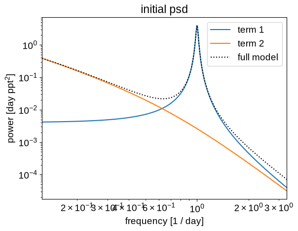
Let’s look at the underlying power spectral density of this initial model:

freq = np.linspace(1.0 / 8, 1.0 / 0.3, 500)
omega = 2 * np.pi * freq


def plot_psd(gp):
    for n, term in enumerate(gp.kernel.terms):
        plt.loglog(freq, term.get_psd(omega), label="term {0}".format(n + 1))
    plt.loglog(freq, gp.kernel.get_psd(omega), ":k", label="full model")
    plt.xlim(freq.min(), freq.max())
    plt.legend()
    plt.xlabel("frequency [1 / day]")
    plt.ylabel("power [day ppt$^2$]")


plt.title("initial psd")
plot_psd(gp)

And then we can also plot the prediction that this model makes for the missing data and compare it to the truth:

def plot_prediction(gp):
    plt.plot(true_t, true_y, "k", lw=1.5, alpha=0.3, label="data")
    plt.errorbar(t, y, yerr=yerr, fmt=".k", capsize=0, label="truth")

    if gp:
        mu, variance = gp.predict(y, t=true_t, return_var=True)
        sigma = np.sqrt(variance)
        plt.plot(true_t, mu, label="prediction")
        plt.fill_between(true_t, mu - sigma, mu + sigma, color="C0", alpha=0.2)

    plt.xlabel("x [day]")
    plt.ylabel("y [ppm]")
    plt.xlim(0, 10)
    plt.ylim(-2.5, 2.5)
    plt.legend()


plt.title("initial prediction")
plot_prediction(gp)

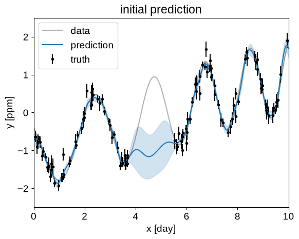
Ok, that looks pretty terrible, but we can get a better fit by numerically maximizing the likelihood as described in the following section.

Maximum likelihood

In this section, we’ll improve our initial GP model by maximizing the likelihood function for the parameters of the kernel, the mean, and a “jitter” (a constant variance term added to the diagonal of our covariance matrix). To do this, we’ll use the numerical optimization routine from scipy:

from scipy.optimize import minimize


def set_params(params, gp):
    gp.mean = params[0]
    theta = np.exp(params[1:])
    gp.kernel = terms.SHOTerm(
        sigma=theta[0], rho=theta[1], tau=theta[2]
    ) + terms.SHOTerm(sigma=theta[3], rho=theta[4], Q=0.25)
    gp.compute(t, diag=yerr**2 + theta[5], quiet=True)
    return gp


def neg_log_like(params, gp):
    gp = set_params(params, gp)
    return -gp.log_likelihood(y)


initial_params = [0.0, 0.0, 0.0, np.log(10.0), 0.0, np.log(5.0), np.log(0.01)]
soln = minimize(neg_log_like, initial_params, method="L-BFGS-B", args=(gp,))
opt_gp = set_params(soln.x, gp)
soln

  message: CONVERGENCE: REL_REDUCTION_OF_F_<=_FACTR*EPSMCH
  success: True
   status: 0
      fun: -15.94282638406871
        x: [ 4.596e-03 -3.416e-01  7.000e-01  1.944e+00  6.059e-01
             3.755e+00 -7.873e+00]
      nit: 52
      jac: [-4.263e-05 -2.714e-04 -1.990e-05  6.253e-05  3.837e-05
             2.132e-05  3.695e-05]
     nfev: 464
     njev: 58
 hess_inv: <7x7 LbfgsInvHessProduct with dtype=float64>

Now let’s make the same plots for the maximum likelihood model:

plt.figure()
plt.title("maximum likelihood psd")
plot_psd(opt_gp)

plt.figure()
plt.title("maximum likelihood prediction")
plot_prediction(opt_gp)

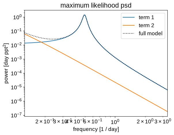
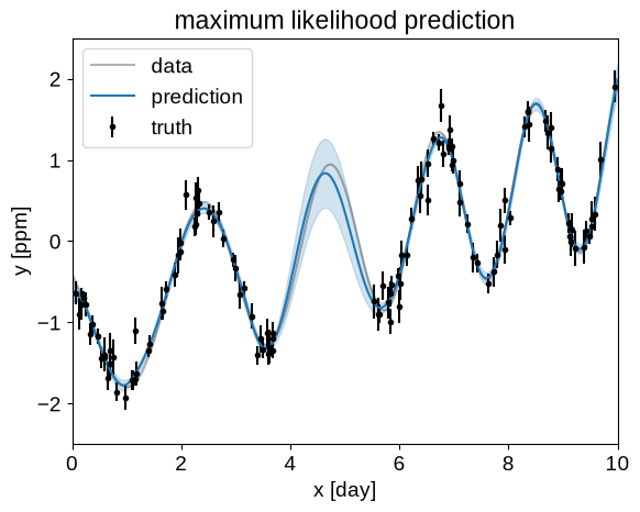
These predictions are starting to look much better!

Posterior inference using emcee

Now, to get a sense for the uncertainties on our model, let’s use Markov chain Monte Carlo (MCMC) to numerically estimate the posterior expectations of the model. In this first example, we’ll use the emcee package to run our MCMC. Our likelihood function is the same as the one we used in the previous section, but we’ll also choose a wide normal prior on each of our parameters.

import emcee

prior_sigma = 2.0


def log_prob(params, gp):
    gp = set_params(params, gp)
    return (
        gp.log_likelihood(y) - 0.5 * np.sum((params / prior_sigma) ** 2),
        gp.kernel.get_psd(omega),
    )


np.random.seed(5693854)
coords = soln.x + 1e-5 * np.random.randn(32, len(soln.x))
sampler = emcee.EnsembleSampler(
    coords.shape[0], coords.shape[1], log_prob, args=(gp,)
)
state = sampler.run_mcmc(coords, 2000, progress=False)
sampler.reset()
state = sampler.run_mcmc(state, 5000, progress=False)

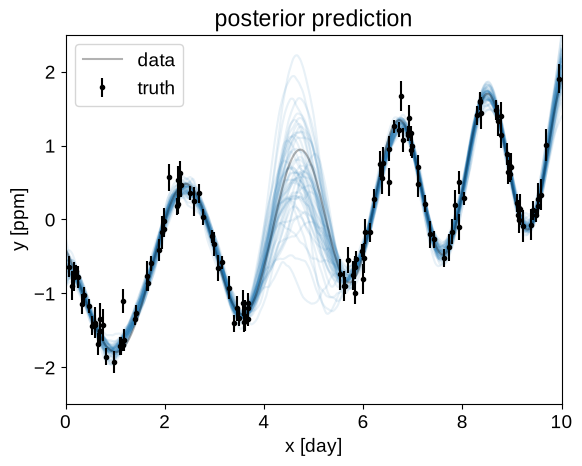
After running our MCMC, we can plot the predictions that the model makes for a handful of samples from the chain. This gives a qualitative sense of the uncertainty in the predictions.

chain = sampler.get_chain(discard=100, flat=True)

for sample in chain[np.random.randint(len(chain), size=50)]:
    gp = set_params(sample, gp)
    conditional = gp.condition(y, true_t)
    plt.plot(true_t, conditional.sample(), color="C0", alpha=0.1)

plt.title("posterior prediction")
plot_prediction(None)

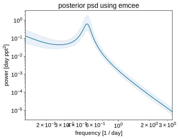
Similarly, we can plot the posterior expectation for the power spectral density:

psds = sampler.get_blobs(discard=100, flat=True)

q = np.percentile(psds, [16, 50, 84], axis=0)

plt.loglog(freq, q[1], color="C0")
plt.fill_between(freq, q[0], q[2], color="C0", alpha=0.1)

plt.xlim(freq.min(), freq.max())
plt.xlabel("frequency [1 / day]")
plt.ylabel("power [day ppt$^2$]")
_ = plt.title("posterior psd using emcee")

Posterior inference using PyMC

celerite2 also includes support for probabilistic modeling using PyMC (v5 or v3, using the celerite2.pymc or celerite2.pymc3 submodule respectively), and we can implement the same model from above as follows:

import pymc as pm
from celerite2.pymc import GaussianProcess, terms as pm_terms

with pm.Model() as model:
    mean = pm.Normal("mean", mu=0.0, sigma=prior_sigma)
    log_jitter = pm.Normal("log_jitter", mu=0.0, sigma=prior_sigma)

    log_sigma1 = pm.Normal("log_sigma1", mu=0.0, sigma=prior_sigma)
    log_rho1 = pm.Normal("log_rho1", mu=0.0, sigma=prior_sigma)
    log_tau = pm.Normal("log_tau", mu=0.0, sigma=prior_sigma)
    term1 = pm_terms.SHOTerm(
        sigma=pm.math.exp(log_sigma1),
        rho=pm.math.exp(log_rho1),
        tau=pm.math.exp(log_tau),
    )

    log_sigma2 = pm.Normal("log_sigma2", mu=0.0, sigma=prior_sigma)
    log_rho2 = pm.Normal("log_rho2", mu=0.0, sigma=prior_sigma)
    term2 = pm_terms.SHOTerm(
        sigma=pm.math.exp(log_sigma2), rho=pm.math.exp(log_rho2), Q=0.25
    )

    kernel = term1 + term2
    gp = GaussianProcess(kernel, mean=mean)
    gp.compute(t, diag=yerr**2 + pm.math.exp(log_jitter), quiet=True)
    gp.marginal("obs", observed=y)

    pm.Deterministic("psd", kernel.get_psd(omega))

    trace = pm.sample(
        tune=1000,
        draws=1000,
        target_accept=0.9,
        init="adapt_full",
        cores=2,
        chains=2,
        random_seed=34923,
    )

WARNING (pytensor.tensor.blas): Using NumPy C-API based implementation for BLAS functions.

/home/docs/checkouts/readthedocs.org/user_builds/celerite2/envs/latest/lib/python3.10/site-packages/tqdm/auto.py:21: TqdmWarning: IProgress not found. Please update jupyter and ipywidgets. See https://ipywidgets.readthedocs.io/en/stable/user_install.html
  from .autonotebook import tqdm as notebook_tqdm

Auto-assigning NUTS sampler...

Initializing NUTS using adapt_full...

/home/docs/checkouts/readthedocs.org/user_builds/celerite2/envs/latest/lib/python3.10/site-packages/pymc/step_methods/hmc/quadpotential.py:627: UserWarning: QuadPotentialFullAdapt is an experimental feature
  warnings.warn("QuadPotentialFullAdapt is an experimental feature")

Multiprocess sampling (2 chains in 2 jobs)

NUTS: [mean, log_jitter, log_sigma1, log_rho1, log_tau, log_sigma2, log_rho2]

/home/docs/.asdf/installs/python/3.10.13/lib/python3.10/multiprocessing/popen_fork.py:66: RuntimeWarning: os.fork() was called. os.fork() is incompatible with multithreaded code, and JAX is multithreaded, so this will likely lead to a deadlock.
  self.pid = os.fork()

/home/docs/checkouts/readthedocs.org/user_builds/celerite2/envs/latest/lib/python3.10/site-packages/rich/live.py:23
1: UserWarning: install "ipywidgets" for Jupyter support
  warnings.warn('install "ipywidgets" for Jupyter support')

/home/docs/.asdf/installs/python/3.10.13/lib/python3.10/multiprocessing/popen_fork.py:66: RuntimeWarning: os.fork() was called. os.fork() is incompatible with multithreaded code, and JAX is multithreaded, so this will likely lead to a deadlock.
  self.pid = os.fork()

Sampling 2 chains for 1_000 tune and 1_000 draw iterations (2_000 + 2_000 draws total) took 26 seconds.

There were 1 divergences after tuning. Increase `target_accept` or reparameterize.

We recommend running at least 4 chains for robust computation of convergence diagnostics

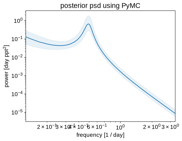
Like before, we can plot the posterior estimate of the power spectrum to show that the results are qualitatively similar:

psds = trace.posterior["psd"].values

q = np.percentile(psds, [16, 50, 84], axis=(0, 1))

plt.loglog(freq, q[1], color="C0")
plt.fill_between(freq, q[0], q[2], color="C0", alpha=0.1)

plt.xlim(freq.min(), freq.max())
plt.xlabel("frequency [1 / day]")
plt.ylabel("power [day ppt$^2$]")
_ = plt.title("posterior psd using PyMC")

Posterior inference using numpyro

Since celerite2 also includes support for JAX, you can also use tools like numpyro for inference.

from jax import config

config.update("jax_enable_x64", True)

from jax import random
import jax.numpy as jnp

import numpyro
import numpyro.distributions as dist
from numpyro.infer import MCMC, NUTS

import celerite2.jax
from celerite2.jax import terms as jax_terms


def numpyro_model(t, yerr, y=None):
    mean = numpyro.sample("mean", dist.Normal(0.0, prior_sigma))
    log_jitter = numpyro.sample("log_jitter", dist.Normal(0.0, prior_sigma))

    log_sigma1 = numpyro.sample("log_sigma1", dist.Normal(0.0, prior_sigma))
    log_rho1 = numpyro.sample("log_rho1", dist.Normal(0.0, prior_sigma))
    log_tau = numpyro.sample("log_tau", dist.Normal(0.0, prior_sigma))
    term1 = jax_terms.SHOTerm(
        sigma=jnp.exp(log_sigma1), rho=jnp.exp(log_rho1), tau=jnp.exp(log_tau)
    )

    log_sigma2 = numpyro.sample("log_sigma2", dist.Normal(0.0, prior_sigma))
    log_rho2 = numpyro.sample("log_rho2", dist.Normal(0.0, prior_sigma))
    term2 = jax_terms.SHOTerm(
        sigma=jnp.exp(log_sigma2), rho=jnp.exp(log_rho2), Q=0.25
    )

    kernel = term1 + term2
    gp = celerite2.jax.GaussianProcess(kernel, mean=mean)
    gp.compute(t, diag=yerr**2 + jnp.exp(log_jitter), check_sorted=False)

    numpyro.sample("obs", gp.numpyro_dist(), obs=y)
    numpyro.deterministic("psd", kernel.get_psd(omega))


nuts_kernel = NUTS(numpyro_model, dense_mass=True)
mcmc = MCMC(
    nuts_kernel,
    num_warmup=1000,
    num_samples=1000,
    num_chains=2,
    progress_bar=False,
)
rng_key = random.PRNGKey(34923)
%time mcmc.run(rng_key, t, yerr, y=y)

/tmp/ipykernel_1038/987984401.py:42: UserWarning: There are not enough devices to run parallel chains: expected 2 but got 1. Chains will be drawn sequentially. If you are running MCMC in CPU, consider using `numpyro.set_host_device_count(2)` at the beginning of your program. You can double-check how many devices are available in your system using `jax.local_device_count()`.
  mcmc = MCMC(

CPU times: user 11.8 s, sys: 156 ms, total: 12 s
Wall time: 11.9 s

This runtime was similar to the PyMC result from above, and (as we’ll see below) the convergence is also similar. Any difference in runtime will probably disappear for more computationally expensive models, but this interface is looking pretty great here!

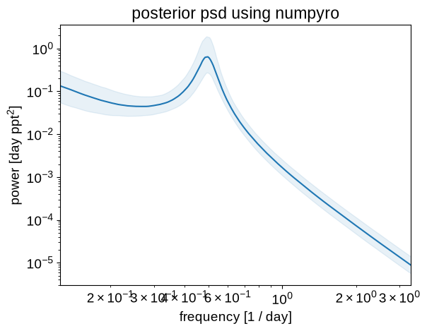
As above, we can plot the posterior expectations for the power spectrum:

psds = np.asarray(mcmc.get_samples()["psd"])

q = np.percentile(psds, [16, 50, 84], axis=0)

plt.loglog(freq, q[1], color="C0")
plt.fill_between(freq, q[0], q[2], color="C0", alpha=0.1)

plt.xlim(freq.min(), freq.max())
plt.xlabel("frequency [1 / day]")
plt.ylabel("power [day ppt$^2$]")
_ = plt.title("posterior psd using numpyro")

Comparison

Finally, let’s compare the results of these different inference methods a bit more quantitaively. First, let’s look at the posterior constraint on the period of the underdamped harmonic oscillator, the effective period of the oscillatory signal.

import arviz as az

emcee_data = az.from_emcee(
    sampler,
    var_names=[
        "mean",
        "log_sigma1",
        "log_rho1",
        "log_tau",
        "log_sigma2",
        "log_rho2",
        "log_jitter",
    ],
)

pm_data = trace
numpyro_data = az.from_numpyro(mcmc)

bins = np.linspace(1.5, 2.75, 25)
plt.hist(
    np.exp(np.asarray((emcee_data.posterior["log_rho1"].T)).flatten()),
    bins,
    histtype="step",
    density=True,
    label="emcee",
)
plt.hist(
    np.exp(np.asarray((pm_data.posterior["log_rho1"].T)).flatten()),
    bins,
    histtype="step",
    density=True,
    label="PyMC",
)
plt.hist(
    np.exp(np.asarray((numpyro_data.posterior["log_rho1"].T)).flatten()),
    bins,
    histtype="step",
    density=True,
    label="numpyro",
)
plt.legend()
plt.yticks([])
plt.xlabel(r"$\rho_1$")
_ = plt.ylabel(r"$p(\rho_1)$")

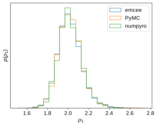
That looks pretty consistent.

Next we can look at the ArviZ summary for each method to see how the posterior expectations and convergence diagnostics look.

az.summary(
    emcee_data,
    var_names=[
        "mean",
        "log_sigma1",
        "log_rho1",
        "log_tau",
        "log_sigma2",
        "log_rho2",
        "log_jitter",
    ],
)

	mean	sd	hdi_3%	hdi_97%	mcse_mean	mcse_sd	ess_bulk	ess_tail	r_hat
mean	-0.006	1.257	-2.491	2.451	0.034	0.024	1627.0	3418.0	1.02
log_sigma1	-0.297	0.331	-0.869	0.338	0.008	0.005	1865.0	3584.0	1.02
log_rho1	0.701	0.059	0.591	0.810	0.001	0.001	1782.0	4277.0	1.02
log_tau	1.889	0.753	0.569	3.337	0.019	0.013	1680.0	3647.0	1.02
log_sigma2	0.524	0.655	-0.608	1.769	0.016	0.012	1608.0	3082.0	1.02
log_rho2	3.322	0.884	1.759	4.981	0.022	0.015	1650.0	4081.0	1.02
log_jitter	-5.829	0.723	-7.180	-4.559	0.020	0.014	1427.0	2897.0	1.02

az.summary(
    pm_data,
    var_names=[
        "mean",
        "log_sigma1",
        "log_rho1",
        "log_tau",
        "log_sigma2",
        "log_rho2",
        "log_jitter",
    ],
)

	mean	sd	hdi_3%	hdi_97%	mcse_mean	mcse_sd	ess_bulk	ess_tail	r_hat
mean	-0.009	1.224	-2.288	2.511	0.037	0.028	1193.0	1124.0	1.0
log_sigma1	-0.288	0.331	-0.878	0.313	0.009	0.006	1571.0	1053.0	1.0
log_rho1	0.702	0.059	0.604	0.816	0.002	0.002	1097.0	600.0	1.0
log_tau	1.924	0.753	0.510	3.283	0.020	0.015	1539.0	1176.0	1.0
log_sigma2	0.510	0.660	-0.637	1.743	0.019	0.016	1418.0	997.0	1.0
log_rho2	3.302	0.878	1.697	4.848	0.025	0.018	1315.0	1212.0	1.0
log_jitter	-5.840	0.753	-7.275	-4.501	0.022	0.016	1460.0	951.0	1.0

az.summary(
    numpyro_data,
    var_names=[
        "mean",
        "log_sigma1",
        "log_rho1",
        "log_tau",
        "log_sigma2",
        "log_rho2",
        "log_jitter",
    ],
)

	mean	sd	hdi_3%	hdi_97%	mcse_mean	mcse_sd	ess_bulk	ess_tail	r_hat
mean	0.031	1.225	-2.541	2.301	0.035	0.032	1349.0	1013.0	1.0
log_sigma1	-0.286	0.351	-0.942	0.373	0.009	0.006	1785.0	1087.0	1.0
log_rho1	0.700	0.055	0.598	0.810	0.001	0.001	1772.0	1390.0	1.0
log_tau	1.954	0.771	0.666	3.504	0.021	0.016	1490.0	1250.0	1.0
log_sigma2	0.530	0.652	-0.577	1.772	0.021	0.017	1037.0	1015.0	1.0
log_rho2	3.314	0.863	1.853	4.960	0.028	0.020	1055.0	1094.0	1.0
log_jitter	-5.817	0.744	-7.214	-4.522	0.020	0.015	1651.0	1203.0	1.0

Overall these results are consistent, but the $\hat{R}$ values are a bit high for the emcee run, so I’d probably run that for longer. Either way, for models like these, PyMC and numpyro are generally going to be much better inference tools (in terms of runtime per effective sample) than emcee, so those are the recommended interfaces if the rest of your model can be easily implemented in such a framework.